Data Profiling¶

Luminaire DataExploration implements different exploratory data analysis to detect important information from time series data. This method can be used to impute missing data, detect the set of historical trend changes and change points (steady data shifts) which information can later be leveraged downstream in Luminaire outlier detection models.

Luminaire data exploration and profiling runs two different workflows. The impute only option in profiling performs imputation for any missing data in the input time series and does not run any profiling to generate insights from the input time series.

Note

If duplicate dates dates are present in the input time series, Data profiling processes the data dates by averaging the duplicates and merging them as a single data date.

>>> from luminaire.exploration.data_exploration import DataExploration
>>> data
               raw
index
2020-01-01  1326.0
2020-01-02  1552.0
2020-01-03  1432.0
2020-01-04  1470.0
2020-01-05  1565.0
...            ...
2020-06-03  1934.0
2020-06-04  1873.0
2020-06-05     NaN
2020-06-06  1747.0
2020-06-07  1782.0
>>> de_obj = DataExploration(freq='D')
>>> imputed_data, pre_prc = de_obj.profile(data, impute_only=True)
>>> print(imputed_data)
                    raw
2020-01-01  1326.000000
2020-01-02  1552.000000
2020-01-03  1432.000000
2020-01-04  1470.000000
2020-01-05  1565.000000
...                 ...
2020-06-03  1934.000000
2020-06-04  1873.000000
2020-06-05  1823.804535
2020-06-06  1747.000000
2020-06-07  1782.000000
>>>print(pre_prc)
None

In order to get the data profiling information, the impute only option should be disabled (that is the default option). Disabling the impute only option allows Luminaire to impute missing data along with detecting all the trend changes and the change points in the input time series.

The key utility of Luminaire data profiling is this being a pre-processing step for outlier detection model training. Hence, the user can enable several option to prepare the time series before ingested by the training process. For example, the log transformation option can be enabled for exponential modeling during training. User can also check for the fill rate to constrain the proportion of missing data upto some threshold. Moreover, the pre processed data can also be truncated if there is any change points (data shift) observed.

>>> de_obj = DataExploration(freq='D', data_shift_truncate=True, is_log_transformed=True, fill_rate=0.8)
>>> imputed_data, pre_prc = de_obj.profile(data)
>>> print(pre_prc)
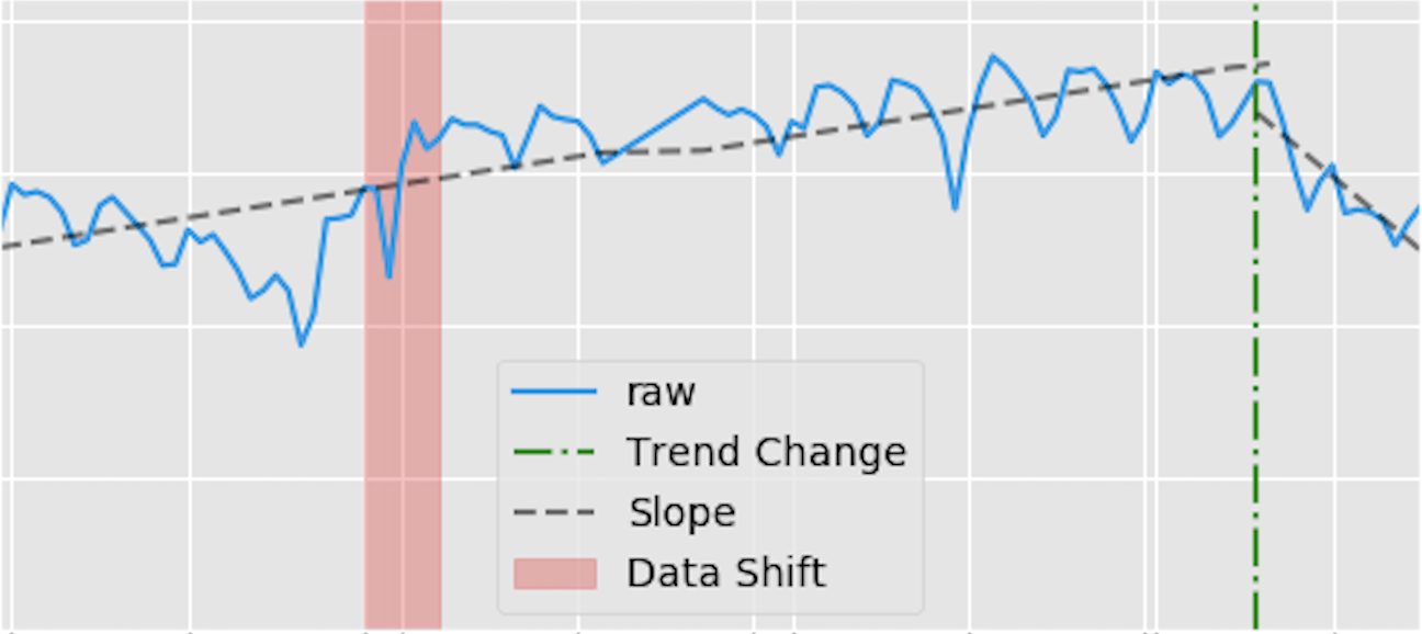
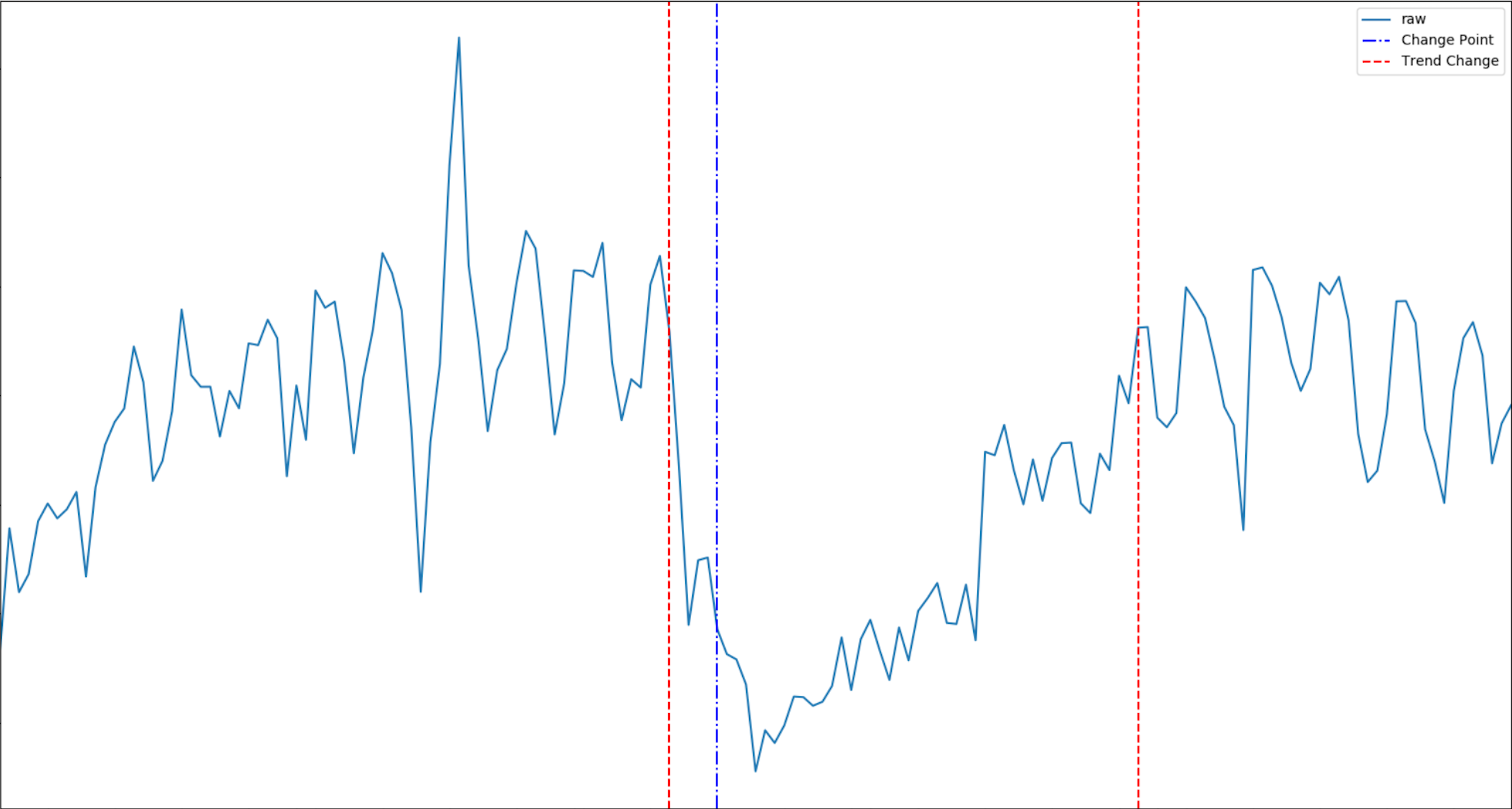
{'success': True, 'trend_change_list': ['2020-04-01 00:00:00'], 'change_point_list': ['2020-03-16 00:00:00'], 'is_log_transformed': 1, 'min_ts_mean': None, 'ts_start': '2020-01-01 00:00:00', 'ts_end': '2020-06-07 00:00:00'}
>>> print(imputed_data)
               raw  interpolated
2020-03-16  1371.0      7.224024
2020-03-17  1325.0      7.189922
2020-03-18  1318.0      7.184629
2020-03-19  1270.0      7.147559
2020-03-20  1116.0      7.018401
...            ...           ...
2020-06-03  1934.0      7.567862
2020-06-04  1873.0      7.535830
2020-06-05     NaN      7.610539
2020-06-06  1747.0      7.466227
2020-06-07  1782.0      7.486052