

Introduction#
Random forests have proven to be very popular and powerful for regression and classification. For regression, random forests give an accurate approximation of the conditional mean of a response variable. That is, if we let \(Y\) be a real-valued response variable and \(X\) a covariate or predictor variable, they estimate \(E(Y | X)\), which can be interpreted as the expected value of the output \(Y\) given the input \(X\).
However random forests provide information about the full conditional distribution of the response variable, not only about the conditional mean. Quantile regression forests, a generalization of random forests, can be used to infer conditional quantiles. That is, they return \(y\) at \(q\) for which \(F(Y=y|X) = q\), where \(q\) is the quantile.
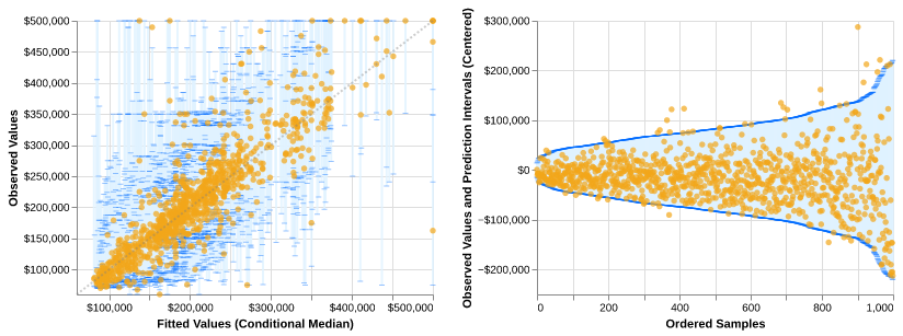
The observed values of houses in California and the 95% prediction intervals that a QRF predicts for them, against the predicted medians (left), and centered and ordered by the width of the interval (right), from Quantile Regression Forests Prediction Intervals.#
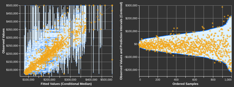
The observed values of houses in California and the 95% prediction intervals that a QRF predicts for them, against the predicted medians (left), and centered and ordered by the width of the interval (right), from Quantile Regression Forests Prediction Intervals.#
The quantiles give more complete information about the distribution of \(Y\) as a function of the predictor variable \(X\) than the conditional mean alone. They can be useful, for example, to build prediction intervals or to perform outlier detection in a high-dimensional dataset.
In practice, the empirical estimation of quantiles can be calculated in several ways. By default, a quantile \(q\) is the smallest training response such that at least a fraction \(q\) of the (weighted) training samples are at or below it, averaged with the next response if exactly that fraction are. Other methods can be specified with the interpolation parameter of the predict method (see the interpolation methods).
Quantile Regression Forests#
A standard decision tree can be extended in a straightforward way to estimate conditional quantiles. When a decision tree is fit, rather than storing only the sufficient statistics of the response variable at the leaf node, such as the mean and variance, all of the response values can be stored with the leaf node. At prediction time, these values can then be used to calculate empirical quantile estimates.
The quantile-based approach can be extended to random forests. To estimate \(F(Y=y|x) = q\), each response value in the training set is given a weight or frequency. Formally, the weight or frequency given to the \(j\)th training sample, \(y_j\), while estimating the quantile is
where \(L(x)\) denotes the leaf that \(x\) falls into.
Informally, this means that given a new unknown sample, we first find the leaf that it falls into for each tree in the ensemble. Each training sample \(y_j\) that falls into the same leaf as the new sample is given a weight that equals the fraction of samples in the leaf. Each \(y_j\) that does not fall into the same leaf as the new sample is given a weight or frequency of zero. The weights or frequencies for each \(y_j\) are then summed or aggregated across all of the trees in the ensemble. This information can then be used to calculate the empirical quantile estimates.
This approach was first proposed by Meinshausen [Mei06]. This package uses these weights if each leaf keeps all of its training samples (max_samples_leaf=None) and weighted_leaves=True (see Fitting and Predicting). By default, each leaf keeps one randomly selected sample (max_samples_leaf=1), so that each tree contributes one response value, and if leaves keep more samples, each sample in a leaf counts once, whatever the size of the leaf (weighted_leaves=False).